Starting with ONETEP
- Author:
Arihant Bhandari, University of Southampton
- Author:
Rebecca J. Clements, University of Southampton
- Author:
Jacek Dziedzic, University of Southampton
- Date:
April 2022 (revised July 2023)
Obtaining a copy of ONETEP
If you are an academic license user, you should have received a tarball of a
personalised ONETEP copy once you have signed an academic licence agreement.
Create a new directory, unpack the tarball there
(tar -xfz your_tarball_name.tar.gz), and you’re done. You can now go
straight to Compiling, testing and running ONETEP.
If you plan to have continuous access to the current ONETEP source code, likely because you are a ONETEP developer or contributor, or collaborate with one, you will want to have access to the official ONETEP GitHub repository.
Take a look at Repository location and structure and ONETEP GitHub set-up to get acquainted with the overall set-up.
If you don’t have a GitHub account yet, follow the steps at Creating a GitHub user account to create one.
Then, create a GitHub personal access token by following the steps at Creating a GitHub personal access token (PAT). Without it you will not be able to access the repository due to GitHub policies (unless you already have a PAT).
Follow Getting access to the ONETEP repository to get access. Be sure to follow further instuctions there, depending on whether you plan to be a User or a Contributor. Congratulations, you have your own copy of ONETEP!
Continue along to Compiling, testing and running ONETEP.
Compiling, testing and running ONETEP
These are the instructions for setting the environment prior to compiling ONETEP, for how to compile ONETEP, and how to run quality-check (“QC”) tests that will give you confidence in the robustness of your installation. There are also instructions on how to actually submit (start) your jobs.
These instructions differ depending on your environment (the machine on which you will run ONETEP and the installed software, such as compilers or external libraries). They are provided separately.
Go to the directory with your ONETEP installation.
Change to the
hpc_resourcesdirectory. There you will see a number of well-supported systems, such asArcher2orYoung(and more).If your machine is well-supported by ONETEP, just follow the compilation, testing and running instructions there. For instance, instructions for Iridis5 would be found at hpc_resources/Iridis5/instructions_iridis5.pdf.
If your machine is not in the list of well-supported systems, you will need to adapt one of the existing configs. Look into the subdirectories under
hpc_resourcesand also in theconfigdirectory in your ONETEP installation.
Important point about compiling ONETEP following a git merge:
Warning
If you just updated your ONETEP source via git merge or git pull
(rather than cloning via git clone or unpacking ONETEP from a tarball),
issue a make cleanall before compiling. The script for cascade avoidance
used when making ONETEP can get confused as to what needs to be rebuilt after a
git merge or git pull. If you forget about make cleanall, you
may get an executable that builds correctly but malfunctions in strange ways
(usually producing very unexpected error messages).
Important point about running QC tests:
Warning
Never run the QC tests in the actual repository. Create a copy of your
ONETEP installation directory (e.g. cp -a onetep_jd onetep_jd_qc) and
run the tests in the directory of the copy. Much of the stuff in the install
is not needed to run the tests (e.g. all of src/), but it’s just less
hassle to copy the entire thing than pick out the necessary subdirectories.
Why not run the QC tests in the actual repository? Because they produce
outputs, which can become messy to clean up back to pristine state,
polluting your repository with spurious changes. This becomes more
problematic because symbolic links are used in the QC test suite. Trying
to update your repository via git pull or git fetch may be
tricky when you have unfinished or improperly cleaned up QC tests. Just
don’t run them straight in the repository.
Creating input files
Go to the ONETEP website, onetep.org. There, under Resources
you will find the Tutorials section, which introduces running various kinds of
ONETEP calculations. Take a look at some of the input files at the
bottom of the page. Input files in ONETEP have the .dat file
extension. Should any files get downloaded having a .txt extension,
you will need to rename them to end with .dat.
Input files contain keywords, instructing ONETEP on what calculations to run, and to set the parameters needed to run them. Check out the keywords on the webpage onetep.org/Main/Keywords to see what they mean. If not specified, most of them have default settings, as listed on the webpage.
The keywords come in different types: logical, integer,
real, text, physical and block. Keywords of the type
logical can have a value of T (true) or F (false).
Keywords that are integer and real are numbers. Keywords of
type text are a string of characters (for example a filename).
Keywords of the type physical refer to physical variables, which
come with units such as angstroem, bohr, joule, hartree, etc. A
block indicates more than one line of input, these are often used
for specifying coordinates.
Some of the important keywords to get started are:
task– to choose what main calculation you would like ONETEP to perform, e.g. a single point energy calculation or geometry optimisation. You can run a properties calculation this way, using output files generated from a single point energy calculation or usingtask singlepointand a separate keyworddo_propertiesset toT.xc_functional– to choose how to approximate the exchange-correlation term in the Kohn Sham DFT energy expression.%block lattice_cart– to define the dimensions of the simulation cell.%block positions_abs– to define the atomic positions in Cartesian coordinates.
As can be seen from the example input files, all block keywords must
end with a corresponding endblock. Be default all coordinates are in
atomic units (bohr). To switch to angstroems, add ang in the first
line of the block:
%block positions_absangC 16.521413 15.320039 23.535776O 16.498729 15.308934 24.717249%endblock positions_absThe species and species_pot blocks detail the parameters of the
atoms. Non-orthogonal Generalised Wannier Functions (NGWFs) are used to
model the atomic orbitals. In the species block, the name we give to
each type atom in the system is given first, followed by the element of
the atom, its atomic number, the number of NGWFs to use (use -1 for an
educated guess) and the radius of each NGWF typically around 8.0-10.0
(in bohr) for an accurate calculation. For instance for carbon you might
use:
C C 6 4 8.0
The species_pot block specifies the location of the pseudopotential
used for each element of the system. The standard ONETEP norm-conserving
pseudopotentials (.recpot files) exclude core electrons. Core
electrons are included in .paw files. Some of these can be found in
your repository’s pseudo directory. A complete database of all
pseudopotentials for all elements in the .paw format can be
downloaded from
https://www.physics.rutgers.edu/gbrv/all_pbe_paw_v1.5.tar.gz. There are also
PAWs and pseudopotential (.recpot) files in the utils-devel
repository at https://github.com/onetep-devel/utils-devel.
write
keywords, but no read keywords because the files aren’t available
to read at this stage. Any continuing input files must include the
read keywords. If the input file name isn’t changed upon
continuation, the output file will be overwrite with the results of
the continuation, so make sure to back up files before continuing.write_denskern Twrite_tightbox_ngwfs Tread_denskern Tread_tightbox_ngwfs Twrite_hamiltonian Tread_hamiltonian TRunning ONETEP in parallel environments
ONETEP is typically run on more than one CPU core – whether on a desktop computer, or at a high-performance computing (HPC) facility. This is termed parallel operation. There are two main modes of parallel operation – distributed-memory computing (sometimes termed simply parallelism), and shared-memory computing (sometimes termed concurrency). ONETEP combines both of them, so it will be crucial to understand how they work.
Distributed-memory parallelism (MPI)
In this scenario a collection of individual processes (that is, running instances of a program) work together on the same calculation. The processes can all reside on the same physical machine (often termed node) – e.g. when you run them on your many-core desktop machine – or on separate machines (nodes) – e.g. when you run them at an HPC facility.
In both cases processes reside in separate memory spaces, which is a fancy way of saying they do not share memory – each of them gets a chunk of memory and they don’t know what the other processes have in their chunks. Yes, even when they are on the same machine.
The problem they work on has to be somehow subdivided between them – this is known as parallel decomposition. One common way of doing that – and one that ONETEP employs – is data decomposition, where it’s the data in the problem that is subdivided across processes. In ONETEP the grids on which quantities like electronic density or external potential are calculated are divided across processes, with each process “owning” a slab of the grid. Similarly, the atoms in the system are divided across processes, with each process “owning” a subset of atoms. Both of these concepts are illustrated in Fig. 1.
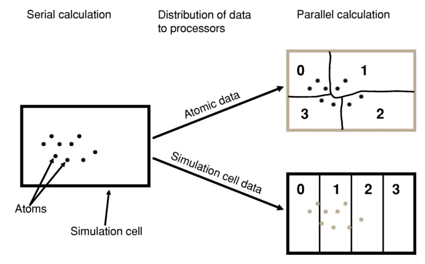
Fig. 1 Illustration of parallel data decomposition in ONETEP. Figure borrowed from J. Chem. Phys. 122, 084119 (2005), https://doi.org/10.1063/1.1839852, which you are well-advised to read.
From the point of view of the operating system, the processes running on a machine are separate entities (see Fig. 2), and collaboration between them almost always necessitates some form of communication (because, remember, they do not share memory) – e.g. process #1 may need to ask process #2 “what are the positions of your atoms?” This is accomplished by a dedicated software library known as Message Passing Interface (MPI). This is why we often call the processes MPI processes, or, more technically, MPI ranks.
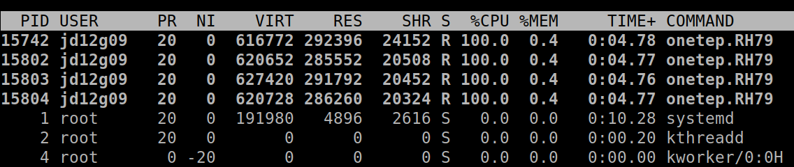
Fig. 2 Four ONETEP processes running on one machine, each utilising 100% of a CPU core and 0.4% of available memory.
MPI facilitates starting multiple processes as part of a single
calculation, which can become slightly tricky when there are multiple
machines (nodes) involved. Your MPI installation will provide a
dedicated command for running multiple processes. The command is often
called mpirun, aprun, gerun, srun or something similar
(it will certainly be stated in the documentation for your system). On a
desktop machine its invocation typically looks like this:
mpirun -np 4 ./onetep_launcher input.dat >input.out 2>input.err
Here, mpirun is the name of the command for launching multiple
processes, -np 4 asks for four processes, onetep_launcher is the name of
the script for launching ONETEP – it’s the script that will actually be
run on four CPU cores, and each instance will start one ONETEP process
for you – here we assume it’s in the current directory (./),
input.dat is your ONETEP input file. Output will be sent
(“redirected”) to onetep.out, and error messages (if any), will be
redirected to input.err. All four processes will be started on the
same machine.
In HPC environments the syntax will be slightly different, because the
number of processes will be automatically inferred by the batch
(queueing) system, the batch system will also take care of instructing
mpirun (or equivalent) what machines to put the processes on.
MPI lets you run your calculation on as many processes as you like – even tens of thousands. However, there are practical limitations to how far you can go with ONETEP. Looking at Fig. 1 it becomes clear that you cannot have more MPI processes than atoms – or some processes would be left without work to do. In fact this limitation is even slightly stricter – to divide work more evenly ONETEP tries to give each processes a similar number of NGWFs, not atoms. For instance, for a water molecule run on two processes, it makes sense to assign the O atom and its 4 NGWFs to one process, and both H atoms (1 NGWF each) to the second process. If you try to run a calculation on H:sub:`2`O on three processes, it’s very likely that ONETEP will do the same thing – assign O to one processes, both H’s to another process and the third process will wind up with no atoms. This will cause the calculation to abort. So, one limitation is you will not be able to use more MPI processes that you have atoms in your system, and even slightly smaller numbers of MPI processes might not work. Even if they do, you don’t really want that, because load balancing will be rather poor – the processor that gets the O atom has roughly twice as much work to do as the one that gets the two H atoms. The bottom line is – you should have at least several atoms per MPI rank – in the interest of efficiency.
Shared-memory parallelism (OMP)
This approach, sometimes known as concurrency, concurrent processing
or colloquially as threads, uses shared memory. The way it works is
a process spawns (starts) a number of threads of execution, with
each thread delegated to a separate CPU core. Typically each thread
works with a subset of data, and, in contrast to processes, threads
within the same process can access each other’s memory. For example, if
a process was given 50 atoms to work with, it can spawn 4 threads and
tell each thread to work on 12-13 atoms. Because threads share memory,
they do not need special mechanisms to communicate – they can just use
memory for this. What they need instead are special mechanisms for
synchronisation – e.g. so that thread 1 knows thread 2 finished writing
something to memory and it’s safe to try to read it. These mechanisms
are described by a standard known as OpenMP, or OMP for short.
In ONETEP threads are most conveniently handled using the launcher’s
-t option, which instructs it how many threads each process should
spawn. For instance the command
./onetep_launcher -t 8 input.dat >input.out 2>input.err
runs one process (note the absence of mpirun), which spawns eight
threads. This is what it looks like to the operating system:

Fig. 3 One ONETEP process that spawned eight threads, running on one machine, utilising almost 800% of a CPU core and 1.3% of available memory – this is for the entire process encompassing eight threads.
Thread-based processing has a number of limitations. As threads reside within a process, you cannot feasibly run more threads than you have CPU cores on a node – in other words, threading is limited to a single node. Moreover, large numbers of threads quickly become inefficient. If a processes owns 10 atoms, using more than 10 threads will not give you any advantage, because the additional threads will not have anything to work with (fortunately, this does not lead to the calculation aborting, only to some threads idling). Even with four threads you will lose some efficiency, because some threads will get 3 atoms and some only 2. ONETEP works best with about 4-6 threads, unless you are using Hartree-Fock exchange (HFx), which is the most efficient on large thread counts.
Threads are easiest to control via onetep_launcher, which you are
advised to use, but ONETEP also provides keywords for controlling them
manually – these are threads_max, threads_per_fftbox,
threads_num_fftboxes, threads_per_cellfft and
threads_num_mkl. Each of these sets the number of threads spawned
from a single process for some part of ONETEP’s functionality. This is
advanced stuff and will not be covered in this beginners’ document.
Another point to note is that each thread requires its own stack (a
region of memory for intermediate data) in addition to the global
(per-process) stack. This per-thread stack needs to be large enough –
almost always 64 MB suffices. So, if you spawn 16 threads from a
process, that’s an extra 1024 MB of memory that you need, per process.
If you use onetep_launcher, it takes care of setting this stack for
you. If you don’t – you’ll need to take care of this on your own (by
exporting a suitable OMP_STACKSIZE) or you risk ugly crashes when
the stack runs out. Not recommended.
Hybrid (combined MPI+OMP) parallelism
For anything but the smallest of systems, combining MPI processes with
OMP threads is the most efficient approach. This is known as hybrid
parallelism. In ONETEP this is realised simply by combining mpirun
(or equivalent) with onetep_launcher’s -t option, like this:
mpirun -np 4 ./onetep_launcher -t 8 input.dat >input.out 2>input.err
Here we are starting 4 processes, each of which spawns 8 threads. This set-up would fully saturate a large, 32-core desktop machine.
Setting up processes and threads looks slightly different in HPC
systems, where you need to start them on separate nodes. Your submission
script (you will find ones for common architectures in the
hpc_resources directory of your ONETEP installation) defines all the
parameters at the top of the script and then accordingly invokes
mpirun (or equivalent) and onetep_launcher. Look at the
beginning of the script to see what I mean.
How many nodes, processes and threads should I use?
There are a few points worth considering here. First of all, efficiency almost universally decreases with the number of CPU cores assigned to a problem. That is to say, throwing 100 cores at a problem is likely to reduce the time to solution by less than 100-fold. This is because of communication overheads, load imbalance and small sections of the algorithm that remain sequential, and is formally known as Amdahl’s law. It’s worth keeping this in mind if you have a large number of calculations to perform (known as task farming) – if you have 1000 calculations to perform, and have 500 CPU cores at your disposal, time to solution will be the shortest if you run 500 1-core jobs first, followed by 500 1-core jobs next. If you opt for running a job on 500 CPU cores simultaneously, and do this for 1000 jobs in sequence, your time to solution will be much, much worse, because of efficiency diminishing with the number of cores.
Having said that, task farming is not the only scenario in the world. Sometimes you have few jobs, or only one, that you want to run quickly. Here, you’re not overly worried about efficiency – if running the job on 1 CPU core takes a month, and using 100 CPU cores reduces it to a day, you’d still take 100 CPU cores, or even more. You just have to remember that the returns will be diminishing with each CPU core you add [1].
The remaining points can be summarised as follows:
Avoid using 1-2 atoms per MPI process, unless there’s no other way. Try to have at least several atoms per MPI process – for good load-balancing.
For OMP threads the sweet spot is typically 4-5 threads. If you have a giant system, so that you have a hundred atoms or more per MPI process, you might be better off using 2 threads or even 1 (using purely distributed-memory parallelism). This is because load balancing will be very good with high numbers of atoms per MPI process. If you have a small system, or if already using large numbers of MPI processes, so that you wind up with very few atoms per MPI process (say, below 5), you might find that using higher numbers of threads (say, 8) to reduce the number of MPI processes is beneficial.
Know how many CPU cores you have on a node. Make sure the number of MPI processes per node and OMP threads per process saturate all the node’s cores. For instance, if you have 40 CPU cores on a node, you should aim for 10 processes per node, 4 threads each; or 20 processes per node, 2 threads each; or 40 processes per node, 1 thread each; or 4 processes per node, 10 threads each. 2 processes per node with 20 threads each would also work, but would likely be suboptimal. Just don’t do things like 3 processes with 10 threads, because then you leave 10 CPU cores idle, and don’t do things like 6 processes with 10 threads, because you then oversubscribe the node (meaning you have more threads than CPU cores) – this degrades performance.
Nodes are often divided internally into NUMA regions – most often there are two NUMA regions per node. The only thing you need to know about NUMA regions is that you don’t want a process to span across them. This is why in the example above you did not see 5 processes with 8 OMP threads each or 8 processes with 5 OMP threads each – I assumed there are two NUMA regions with 20 CPU cores each. In both examples here you would have a process spanning across two NUMA regions. It works, but is much slower.
Points 1-3 above do not apply to Hartree-Fock exchange calculations. Point 4 applies. When doing HFx calculations (this includes calculations with hybrid exchange-correlation functionals, like B3LYP) follow the more detailed instructions in the HFx manual.
If you find that your calculation is running out of memory, your first step should be to increase the number of nodes (because it splits the problem across a set-up with more total RAM). Another idea is to shift the MPI/OMP balance towards more threads and fewer MPI processes (because this reduces the number of buffers for communication between MPI processes). So if your job runs out of memory on 2 nodes with 10 processes on each and with 4 threads per process, give it 4 or more nodes with 10 processes on each with 4 threads per each, or switch to 4 processes with 10 OMP threads.